项目背景:
客户是一个电影制作的新公司,他们将制作一部新电影。客户想确保电影能够成功,从而使新公司立足市场。
提出问题:
- 电影类型是如何随着时间的推移发生变化的?
- Universal Pictures 和 Paramount Pictures
之间的对比情况如何? - 改编电影和原创电影的对比情况如何?
- 电影页面查看次数与评分次数的相关关系?
理解数据:
数据来源
数据来源于Kaggle项目数据
TMDB 5000 Movie Dataset
导入数据
    import numpy as np # linear algebra
    import pandas as pd # data processing, CSV file I/O (e.g. pd.read_csv)

    moviesDf = pd.read_csv("../input/tmdb_5000_movies.csv")
    creditsDf = pd.read_csv("../input/tmdb_5000_credits.csv")
    moviesDf.head(2)
    creditsDf.head()
观察得知,movies中的id列和credits中的movie_id列呈对应关系,因此链接合并两个数据集。
    fullDf = pd.merge(moviesDf,creditsDf,right_on=\'movie_id\',left_on=\'id\',how=\'left\')
    fullDf.head(2)
查看数据集的行列数,描述统计信息,缺失情况,各列数据类型
    # fullDf.shape //查看数据集行列数
    # fullDf.describe() //描述统计情况,查看最小值,异常值
    fullDf.info() //查看缺失值情况,以及各列的数据类型
经观察,budget、vote_count、
vote_average、revenue最小值为0,列中可能有异常值;homepage、overview、release_date、runtime、tagline列均有数据缺失
数据清洗
数据预处理
- 选择子集
选择需要进行分析的数据列作为数据子集 - 列名重命名
    fullDf = fullDf[[\'id\',\'popularity\',\'budget\',\'revenue\',\'original_language\',\'spoken_languages\',\'cast\',\'crew\',\'title_x\',\'status\',\'keywords\',\'runtime\',\'genres\',\'production_companies\',\'release_date\',\'vote_count\',\'vote_average\']]
    titleDict={\'title_x\':\'title\'}
    fullDf.rename(columns=titleDict,inplace=True)
- 缺失数据处理
    fullDf.loc[fullDf["release_date"].isnull(),\'title\']
    fullDf[\'release_date\'] = fullDf[\'release_date\'].fillna(\'2014-06-01\') #查询到空白数据的实际上映时间
    fullDf[\'runtime\'] = fullDf[\'runtime\'].fillna(fullDf[\'runtime\'].mean()) #均值填充
- 数据类型转换
将json格式的字符串转换为python格式的字符串
在这里遇到了很多问题,如json.load()和json.loads()的区别
json.loads()
将json格式的字符串解码转换成Python对象
json.dumps()
实现python类型转换为json字符串,返回一个str对象
json.dump()
将python内置类型序列化为json对象后写入文件
json.load()
读取json形式的字符串元素,转换为python类型
    import json
    json_col = [\'genres\',\'keywords\',\'crew\',\'production_companies\',\'production_countries\',\'spoken_languages\',\'cast\']
    for i in json_col:
        fullDf[i]=fullDf[i].apply(json.loads)
    for index,i in zip(fullDf.index,fullDf[\'genres\']):
        list1=[]
        for j in range(len(i)):
            list1.append((i[j][\'name\']))
        fullDf.loc[index,\'genres\']=str(list1)
    for index,i in zip(fullDf.index,fullDf[\'keywords\']):
        list1=[]
        for j in range(len(i)):
            list1.append((i[j][\'name\']))
        fullDf.loc[index,\'keywords\']=str(list1)
    for index,i in zip(fullDf.index,fullDf[\'crew\']):
        list1=[]
        for j in range(len(i)):
            list1.append((i[j][\'name\']))
    for index,i in zip(fullDf.index,fullDf[\'production_companies\']):
        list1=[]
        for j in range(len(i)):
            list1.append((i[j][\'name\']))
        fullDf.loc[index,\'production_companies\']=str(list1)
    for index,i in zip(fullDf.index,fullDf[\'production_countries\']):
        list1=[]
        for j in range(len(i)):
            list1.append((i[j][\'name\']))
        fullDf.loc[index,\'production_countries\']=str(list1)
    for index,i in zip(fullDf.index,fullDf[\'spoken_languages\']):
        list1=[]
        for j in range(len(i)):
            list1.append((i[j][\'name\']))
        fullDf.loc[index,\'spoken_languages\']=str(list1)
    for index,i in zip(fullDf.index,fullDf[\'cast\']):
        list1=[]
        for j in range(len(i)):
            list1.append((i[j][\'name\']))
        fullDf.loc[index,\'cast\']=str(list1)
将日期的datetime数据类型转换为日期,并提取出年份月份
    fullDf[\'release_year\']=pd.to_datetime(fullDf[\'release_date\'],format=\'%Y-%m-%d\').dt.year
    fullDf[\'release_month\']=pd.to_datetime(fullDf[\'release_date\'],format=\'%Y-%m-%d\').dt.month
    fullDf.drop(columns=[\'release_date\'])
- 数据排序
按照发行年月进行升序排列
    fullDf=fullDf.sort_values(by=[\'release_year\',\'release_month\'],ascending=\'True\')
    fullDf=fullDf.reset_index(drop=\'True\')
    fullDf.drop(columns=[\'release_date\'])
- 异常值处理
将最小值0用平均值填充
    fullDf[\'budget\']=fullDf[\'budget\'].replace(0,fullDf[\'budget\'].mean())
    fullDf[\'vote_count\']=fullDf[\'vote_count\'].replace(0,fullDf[\'vote_count\'].mean())
    fullDf[\'revenue\']=fullDf[\'revenue\'].replace(0,fullDf[\'revenue\'].mean())
    fullDf[\'vote_average\']=fullDf[\'vote_average\'].replace(0,fullDf[\'vote_average\'].mean())
    fullDf.drop(columns=[\'release_date\'])
提取特征——数据分类
- 数值类型的数据:
id、popularity、budget、revenue、runtime、vote_count、vote_average - 时间序列数据:
release_date,已转换为单独的年份release_year、月份列release_month - 分类数据:
有直接类别的数据:
status,original_language
字符串类型:
spoken_languages、cast、crew、genres、 production_companies、production_countries
构建模型
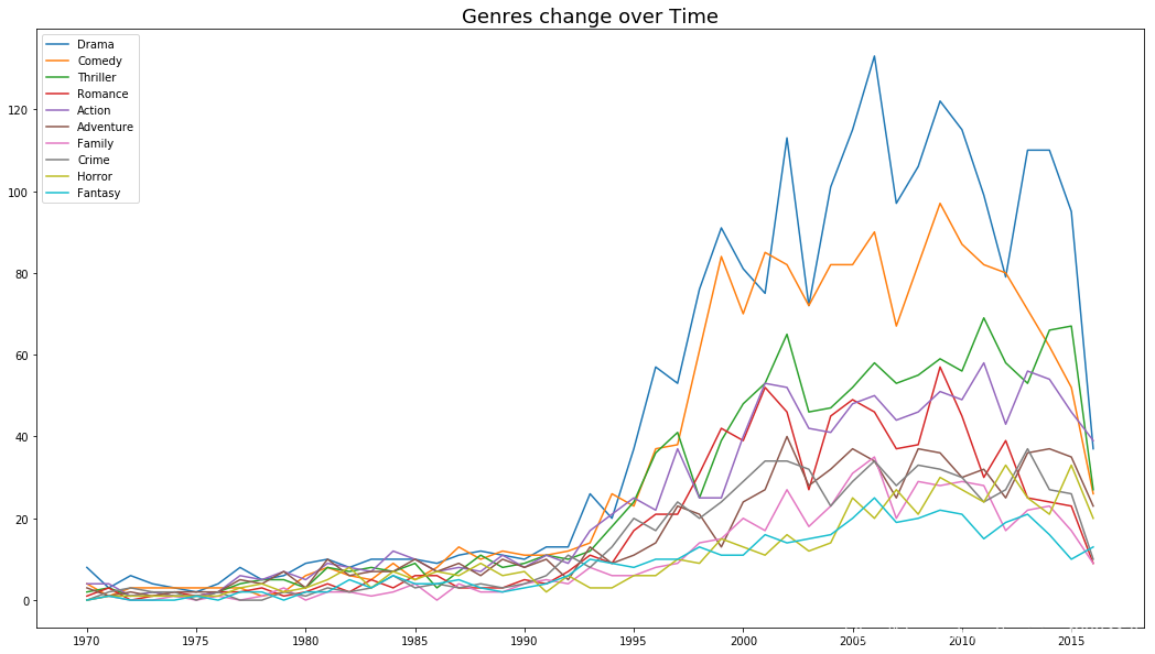
- 电影类型随着时间的推移发生的变化
    #电影类型是如何随着时间的推移发生变化的?
    #选取年份及某种类型电影的数量分别作为X及Y轴
    #提取年份范围
    min_year=fullDf[\'release_year\'].min()
    max_year=fullDf[\'release_year\'].max()
    #提取电影类型
    fullDf[\'genres\']=fullDf[\'genres\'].str.strip(\'[]\').str.replace(\' \',\'\').str.replace("\'",\'\')
    fullDf[\'genres\']=fullDf[\'genres\'].str.split(\',\')
    liste_genres=set()
    for s in fullDf[\'genres\']:
        liste_genres=set().union(s,liste_genres)
    liste_genres=list(liste_genres)
    #构建模型
    genre_df=pd.DataFrame(index=liste_genres,columns=range(min_year,max_year+1))
    genre_df=genre_df.fillna(value=0)
    year=np.array(fullDf[\'release_year\'])
    z=0
    for i in fullDf[\'genres\']:
        split_genre=list(i)
        for j in split_genre:
            genre_df.loc[j,year[z]]=genre_df.loc[j,year[z]]+1
        z+=1
    genre_df
选取数量排在前11名的电影类型,选取1970年以后的数据
    genre_df=genre_df.sort_values(by=2005,ascending=False)
    genre_df=genre_df.iloc[0:10,-48:-1]
    genre_df
    import matplotlib.pyplot as plt
    plt.figure(figsize=(18,10))
    plt.plot(genre_df.T)
    plt.title(\'Genres change over Time\',fontsize=18)
    plt.xticks(range(1970,2020,5))
    plt.legend(genre_df.T)
    plt.show
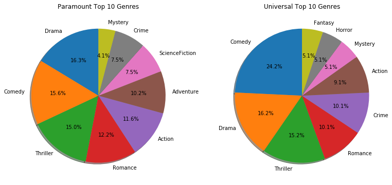
- 比较Universal Pictures和Paramount Pictures两家公司发行的电影类型
    # Universal Pictures和Paramount Pictures之间的对比情况如何?
    # 以两家公司名标记制作公司栏
    for i in fullDf[\'production_companies\']:
        if \'Paramount Pictures\' in i:
            i = \'Paramount Pictures\'
        elif \'Universal Pictures\' in i:
            i = \'Universal Pictures\'
        else:
            i = \'\'
    fullDf[\'production_companies\'] = fullDf[\'production_companies\'].str.strip(\'[]\').str.replace("\'",\'\')
    parDf = fullDf.loc[fullDf[\'production_companies\']==\'Paramount Pictures\']
    uniDf = fullDf.loc[fullDf[\'production_companies\']==\'Universal Pictures\']
    com_gen_df=pd.DataFrame(index=liste_genres,columns=[\'Paramount\',\'Universal\'])
    com_gen_df=com_gen_df.fillna(value=0)
    for i in parDf[\'genres\']:
        split_genre = list(i)
        for j in split_genre:
            com_gen_df.loc[j,\'Paramount\']=com_gen_df.loc[j,\'Paramount\']+1
    for i in uniDf[\'genres\']:
        split_genre = list(i)
        for j in split_genre:
            com_gen_df.loc[j,\'Universal\']=com_gen_df.loc[j,\'Universal\']+1
    com_gen_df.head()
    # 选取排名前10的电影类型
    com_gen_df=com_gen_df.sort_values(by=\'Paramount\',ascending=False)
    Par_gen_df=com_gen_df.iloc[0:9,]
    com_gen_df=com_gen_df.sort_values(by=\'Universal\',ascending=False)
    Uni_gen_df=com_gen_df.iloc[0:9,]
    # 绘图
    fig=plt.figure(\'Paramount VS Universal\',figsize=(13,6))
    ax=fig.add_subplot(121)
    ax.set_title(\'Paramount Top 10 Genres\')
    ax.pie(x=Par_gen_df[\'Paramount\'],labels=Par_gen_df.index,shadow=True,autopct="%1.1f%%",labeldistance=1.1,startangle=90,pctdistance=0.6)
    ax=fig.add_subplot(122)
    ax.set_title(\'Universal Top 10 Genres\')
    ax.pie(x=Uni_gen_df[\'Universal\'],labels=Uni_gen_df.index,shadow=True,autopct="%1.1f%%",labeldistance=1.1,startangle=90,pctdistance=0.6)
    plt.show()
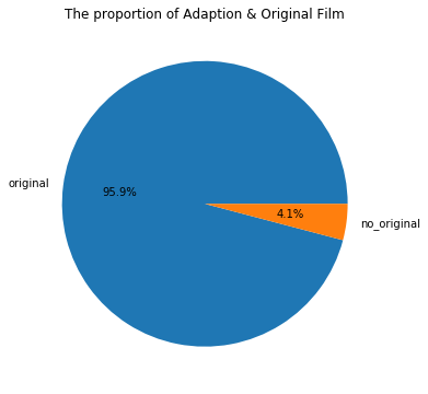
- 原创电影和改编电影之间的对比情况如何?
    # 改编电影adaption和原创电影original对比情况如何
    a=\'based on novel\'
    fullDf[\'if_original\']=fullDf[\'keywords\'].str.contains(a).apply(lambda x:\'no_original\' if x else \'original\')
    key_count=fullDf[\'if_original\'].value_counts()
    plt.figure(figsize=(6,6))
    plt.title(\'The proportion of Adaption & Original Film\')
    plt.pie(x=key_count,labels=key_count.index,labeldistance=1.1,autopct=\'%1.1f%%\')
    plt.show()
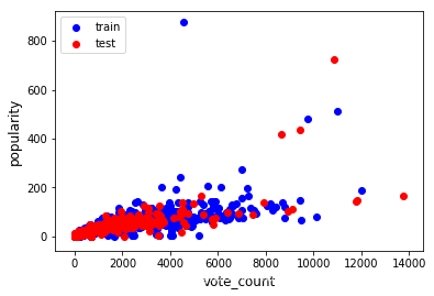
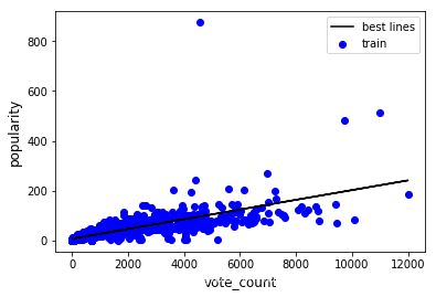
- 评分次数和电影页面查看次数的相关关系如何?
    # 建立模型vote_count与popularity相关系数为0.77
    x = fullDf[\'vote_count\']
    y = fullDf[\'popularity\']
    # 拆分训练数据和测试数据
    from sklearn.model_selection import train_test_split
    x_train,x_test,y_train,y_test=train_test_split(x,y,train_size=0.8)
    plt.scatter(x_train,y_train,color=\'blue\',label=\'train\')
    plt.scatter(x_test,y_test,color=\'red\',label=\'test\')
    plt.xlabel(\'vote_count\',fontsize=12)
    plt.ylabel(\'popularity\',fontsize=12)
    plt.legend(loc=2)
    plt.show()
    # 导入模型
    from sklearn.linear_model import LinearRegression
    x_train=x_train.values.reshape(-1,1)
    x_test=x_test.values.reshape(-1,1)
    trainmodel=LinearRegression()
    trainmodel.fit(x_train,y_train)
    # 最佳拟合线 a=截距 b=回归系数
    a=trainmodel.intercept_
    b=trainmodel.coef_
    print(a,b)
7.769665509560758 [0.01948283]
    plt.scatter(x_train,y_train,color=\'blue\',label=\'train\')
    y_train_pred=trainmodel.predict(x_train)
    plt.plot(x_train,y_train_pred,color=\'black\',label=\'best lines\')
    plt.xlabel(\'vote_count\',fontsize=12)
    plt.ylabel(\'popularity\',fontsize=12)
    plt.legend(loc=1)
    plt.show()
    # 评估模型
    trainmodel.score(x_test,y_test)
0.6055473056494662